Evidence accumulation lab
Introduction
In this lab, we will discuss how computational models are used in cognitive neuroscience, looking at how one class of models, drift diffusion models, are used to express and test hypotheses about visual perception.
Learning goals
After this lab you should have a better understanding of the following:- What models are, and how they are used in cognitive neuroscience
- How drift diffusion models (DDM) work, and what they capture about decision making
- How to use models to make predictions about behavior
What is a computational model?
Computational models are abstract, mathematical descriptions that strip down the thing being described into its essential parts. You already learned about how simple cells, complex cells, and even deep neural networks can be a model for the human visual cortex. Today we're going to go one step further: we'll take a model of human decision making and look at how it can be used to understand both neural activity and human behavior.
Last week we introduced verbal models, for example: "A retinal ganglion cell computes its activity according to the rule: when photons are entering the excitatory regions of its receptive field increase activity and decrease activity when photons enter the inhibitory regions". A computational model takes this concept and turns it into a formal language where the computations are replaced with mathematical formula.
For your thought question this week you played a simple game involving picking whether a patch of motion was moving to the right or to the left. Today you are going to create a computational model for this behavior and then write that model down as a set of mathematical formula. In the thought question we asked you about your subjective experience during the task--a good initial source of insight. Your experience probably differed slightly, but a general verbal model explaining how you solved the task might sound something like this: "To compute whether motion appeared to the left or right an observer tracks many dots simultaneously and keeps track of whether they are consistent in their motion--after accumulating evidence until they feel confident, the observer then makes a choice."
The first step of todays tutorial is to translate this verbal model into a computational one and see whether it explains our results. Please get out the data from your results on the demo and enter them below.
Press enter in each box to submit your data and continue.
Our verbal model is: To compute whether motion appeared to the left or right an observer tracks many dots simultaneously and keeps track of whether they are consistent in their motion--after accumulating evidence until they feel confident, the observer then makes a choice.
We're now going to transform the verbal model into a computational one that we can simulate. The first thing we're going to do is think about the first part of the verbal model "an observer tracks many dots simultaneously and keeps track of whether they are consistent in their motion". What we're going to do is output onto the graph below the observer's belief about the direction of the dots. This happens over time, and at each time step (one millisecond passing), we'll add the current motion strength if the observer sees rightward motion, and subtract it if they see leftward motion.
You can see that depending on whether the motion is to the left or right (click the motion to switch) the graph shoots off in that direction. This is what we call the evidence. The evidence builds up over time so at any given moment the way to think about is that there is X evidence after Y milliseconds have passed, in favor of one direction. Note also that, just like in the task you did, there is a low and high coherence mode. How does evidence accumulate differently in the two conditions?
A question you might have right now is, how much evidence should we be adding on each millisecond? On the last panel we literally added the current coherence value--so for perfectly coherent motion we would have added one and for incoherent motion zero. What's the right value to use?
The answer is that it depends: the reason we're building up this model is that we want to be able to interpret our data. So intuitively the value we use should be fit to the data. Let's do that now. Below there is a slider that controls the drift rate parameter. This parameter is a multiplier: it scales the rate that evidence will grow based on the current coherence.
What we want you to do is change the parameter value until it fits well to your data. You'll see this up top--we're showing you your data which you entered earlier. And in red we're showing you the model. Adjust the parameter until it fits reasonably well. Are you able to fit both the low and high coherence conditions? If not, do you know why: discuss with your neighbor, think about whether the slope of evidence accumulation should be directly related to the actual motion coherence shown? Make a note about whether this fit well or not--we'll discuss it as a group in a moment.
The next step is to add to our model a decision point. Remember we said that the numbers on the left are the evidence so far. How much evidence would you need to be convinced that the motion really went left or right? We call this the decision boundary. We've set the boundary to be +/- 100 and have added these to the plot so you can see them.
There's one last piece missing. What about the trials you got wrong? In the real world there is noise. You should recall (and your data above should remind you) that especially at harder difficulties you occasionally made mistakes. These mistakes happen for a variety of reasons: distractions, brief moments where due to randomness in the dots they appear to go in the wrong direction, etc. To add noise into the model we'll add a small random number to the drift rate at each millisecond. You can control how strong the noise is with the next parameter slider. You should now see that as you increase the noise the model will sometimes end up hitting the wrong boundary, which we count as an incorrect trial. Try adjusting the noise until your percent correct data from the model are similar to your actual results. You might have to adjust the drift rate as well, because the noise and drift rate trade off to some extent.
You may have noticed that it was quite difficult to match up your data to the model. There are a number of reasons for this. One problem is that we used a linear scaling of motion coherence to drift rates. Discuss with your neighbor what a more appropriate relationship might be (for reference low coherence is 15% and high is 65%, if the relationship is linear the "ease" of seeing directions should increase by a factor of four when you go from low to high coherence). Another problem is that it takes your brain a certain amount of time, regardless of the motion coherence, to respond. This is called the non-decision time. We've enabled one last variable for you to try out which controls this time. (Note: the non-decision time isn't being shown on the graph)
Nice work. We've translated the verbal model (from above) into a computational one composed of the drift rate, the noise, and a boundary. You might have noticed that you weren't able to fit your data perfectly--that's okay! In practice model fitting like this is usually done with a lot more data than we had here.
Before we go on we're going to have a group discussion about how you might interpret the parameters that you chose. Please let the TA know you're finished with the first section.
High coherence % correct =
Low coherence reaction time =
High coherence reaction time =
Drift diffusion models (DDMs) in the brain
You should now be familiar with the basics of the drift diffusion model. But remember the model on its own isn't that exciting. The reason we're excited about this and we want you to learn about it is because we think that in some specific tasks the brain operates in a similar way to a drift diffusion model.
The particular task you've been doing has been extensively used by the lab of Professor Bill Newsome here at Stanford: macaques were shown moving dots on a screen, and they had to decide whether the dots were predominantly moving to the left or to the right. The task was made harder or easier by changing the proportion of dots that were moving in concert. This is similar to the task that you've been working with so far.
You now know that by fitting the DDM you can create a model of decision-making as a process where evidence is noisily accumulated in favor of one of two alternatives ("left" or "right"). What does it mean to accumulate evidence in the brain? Well, what Bill Newsome and others suggest is that there might be a decider neuron that is counting the "votes" cast by other, motion-detecting neurons. They've argued that these decider neurons continue to count votes until they hit a threshold and then they fire. We're going to see whether this is true: can a drift diffusion model explain both behavior (which we've seen) and neural activity?
One thing to keep in mind as we go forward is that we will be distinguishing single neurons and populations. A single neuron, as you learned before, may see a feature--but it will have a lot of noise (for example: imagine a neuron whose receptive field is just on the border of the motion "patch" depending on exactly where your eyes are that neuron might respond a lot or not at all). A population of neurons gets around this problem by pooling together many neurons: in a sense it becomes invariant to different sources of noise.
Simulating a neural population
You've already seen in the first lab how a cell can "see" certain kinds of features, even as complex as a dog or a cat, by building up from less complex features. Here what we're going to have are two populations of neurons that respond to rightward or leftward motion, respectively. We're going to walk through this in steps, building up from a single neuron.
First, take a look at this patch of dots. By clicking on the patch you can change it's direction. If you click and drag the slider bar you'll see the motion coherence (% of dots moving) change.
Right preferring population
What you see plotted below is the firing rate of one neuron whose receptive field overlaps with the stimulus. When the motion goes in the preferred direction the firing rate will go up. Note that it is also modulated by the motion coherence. This single neuron is slightly variable--this is due to random noise in the firing rate of the neuron.
You might be asking yourself how does firing rate relate to the spikes you saw in the last tutorial. The answer is that we're plotting here the rate of spiking over time. This is because people believe that rate coding is an important property of how neurons represent information.
Now what you see is the response of many neurons averaged together (the blue line) and many individual neurons (gray lines). Remember that each of the neurons have some variability in the strength of their responses: this causes the population response to inhereit some noise, but importantly the noise in the population is smaller than the noise across the population.
Finally you now see the response of two populations of neurons, one that prefers left motion and one that prefers right.
The purpose of this demonstration was to show how two neural outputs can read out different features from the exact same stimulus.
Simulating a single decision
At this point it's good to point out the parallels between what we're doing here and what we did before. At the beginning you took your behavioral data: percent correct and reaction time, and you tweaked the parameters of the model to fit the data. In the background what happened was that we actually simulated the model: starting at 0 evidence, we added the drift rate plus a bit of random noise at each millisecond. We checked at each step to see whether the model had hit a boundary yet, and if it did then we wrote down the current time (the reaction time) and which boundary we hit (the decision). To get a percent correct for example we would simulate one hundred runs.
In the next section we're going to try to extend the model, which we've used to fit behavioral data, to help understand the MT->LIP circuit. To build up the model we're going to imagine that our macaque brain is looking at a motion patch for a few hundred milliseconds (just like your brain did). This means that the populations of left and right preferring neurons will each be activated to some extent at every moment in time. Their current firing rate will be the evidence accumulated so far.
To visualize what we mean we're going to show you the same motion display as before. Again, you can control the coherence and the direction of the motion. But now we're going to add a new plot below which will have: the firing rate of the left population, right population, and the accumulated evidence in black.
What do we mean by "accumulated evidence"? Well, intuitively, the evidence at any given moment for left is the firing rate of the left population minus the firing rate of the right population. All we do is sum that up over time, as in this equation:
Motion sample
There are a few things to note here.
- First, the black line should look familiar--this is what we were plotting earlier on with your data. The evidence so far.
- Even when you put in the same coherence and direction twice, you get slightly different results. This is due to the noise
- At a glance, the left and right population responses don't give you much information at all. It's only by summing them up that you can tell what direction the patch is going.
At this point it should be quite intuitive that the drift diffusion model fits in well with neural activity. The drift rate is an abstraction of the firing rate of neurons in MT. The noise is just random firing of the neural population. The current evidence corresponds to the firing of neurons in LIP. The boundary is just the threshold where LIP neurons are firing strongly enough to activate muscle output. We're going to take this idea now and use it to fit some neural data.
This slide includes bonus content and is not required.
Bonus content (not required)Simulating a single decision
It's now your turn to write some code! The first thing we're going to do is generate neural population responses based on a motion patch. We're going to give you two numbers: the coherence of the patch (what % of dots are moving together), and the direction. Your job is going to be to complete two functions that will tell us what the neural population response looks like based on what the neurons are seeing (the coherence and direction). Remember that neurons have some response, but they also have noise. We've written a function randn() that we will use to get random numbers pulled from a normal distribution. Try out randn() here: just press enter, you'll see the output of this function below.
Try pressing enter a few more times, you should see that the values you get are being taken from the random normal (gaussian) distribution, centered at 0 with a standard deviation of 1. If you're not familiar with normal distributions this is a good time to ask your neighbor, or the TA, to describe how these work.
Now imagine that we have a motion patch that has some motion coherence and direction. We've stored these values in the variables patch_coherence which can go from 0 to 1 and patch_dir which is either 1 (right) or -1 (left). Use these values to fill out the two functions below: leftResponse() and rightResponse(), so that they return the response of the neural population. Remember the response should be some function of the coherence, plus noise, i.e. as in this equation but where F() is a function that you can pick.
Nice work! You now have two functions leftResponse() and rightResponse() that you'll be able to re-use later. Right now we're going to use them to generate samples like in the graph on the last page. We'll then write one more function to integrate these, and then we'll have our drift-diffusion model!
This slide includes bonus content and is not required.
Simulating a single decision
We're missing two more pieces for our drift diffusion model. The first is that we need to accumulate the evidence over time and the second is that we need to stop accumulating when we hit the threshold. You'll write that code in this next section. If you realize you made a mistake on the previous page you'll be able to go back and edit those as soon as you finish writing these functions.
Fantastic work! It's time to see your code in action! Below what we're doing is the boring part: we start at 0 and we repeat over and over checking what your leftResponse() and rightResponse() functions return given the current stimulus, then we add those up using the acumulateDDM() function, and finally we check whether we should stop using your atThreshold() function. Below we are plotting the output of your code based on the motion coherence and direction of this dot patch. This should look familiar, if you did everything correctly it should look more or less like the plot we showed you earlier.
Motion sample
You should be asking yourself: what happened to the parameters!? We completely ignored them! We'll add them back in later, right now we just want the basic idea of how the code works to you.
This slide includes bonus content and is not required.
Bonus content (not required)Simulating many decisions
The drift diffusion model is most useful as a simulation. Given some set of parameters: a drift rate, diffusion rate, and threshold, the model will create all sorts of different scenarios for how a particular event might play out. But: on average with any given set of parameters we'll get some number of trials that come out correct, some number that are incorrect, and also the reaction time on each trial. You've already seen this in practice when you moved the sliders to fit the model to your own personal data. What we're showing you now is what's happening under the hood.
We're going to model twenty-five trials and just look at the variability in results that we get. Try tweaking the evidence for left or right motion, changing the amount of noise, or changing the thresholds, you'll see the output change each time you change the parameters. Press enter in the input box to re-run the model.
What should be apparent from this simulation is that different diffusion, drift, and threshold parameters can fit all kinds of sets of data (hits, misses, RTs). Recall though that by converting a set of behavioral data into a DDM model fit we gain parameters that are interpretable. What does a hit rate really mean? Not necessarily that much: but what about a drift rate? A lot of research suggests that there are direct neural correlates to the drift diffusion model parameters. In other words if we record from the brain we can find neurons that actually appear to be computing drift diffusion while we make decisions. In the last section we'll look at real recordings from macaque neurons in the lateral intraparietal area and as you'll see we will be able to model them reasonably well using the drift diffusion model.
Fitting to data
In the following image we're going to show you real data recorded from 56 neurons in the macaque lateral intraparietal area (LIP). It's thought that LIP acts as an accumulator of evidence when making decision about direction of motion. The graph is set up similar to how we've shown it before--time is on the X axis but now firing rate is on the Y axis. The hypothesis is that firing rate is representing the accumulated evidence at any given moment in time. You're now going to hand fit a drift diffusion model to see whether the model captures the variance in the data, and if so we'll consider that evidence that the hypothesis might be correct.
The solid lines are from correct trials and dashed lines were incorrect, and each condition was averaged across left and right motion. Notice that the lines break out by motion coherence just as you might expect: stronger motion coherence causes firing rates to peak more quickly.
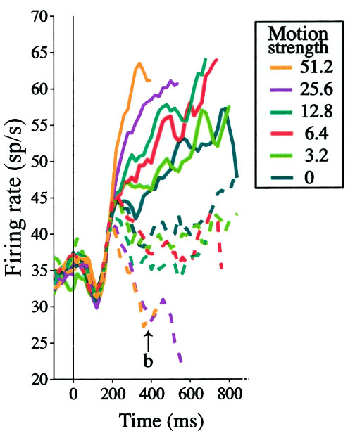
Roitman, J. D., & Shadlen, M. N. (2002).
Like before we're going to let you define how the drift rate, diffusion rate, and threshold, might vary as a function of the motion coherence on each trial. As output we'll show you the data from this graph compared to the average output of 56 trials of your drift diffusion model. Your goal is to minimize the difference between the model output and the data. With your neighbors think about how you would interpret the parameters.
Toggle incorrectAs you try out different approaches think about how well your model fits to the entirety of the data here. If you ignore the incorrect trials how close to reality can you achieve? Adding in the incorrect trials, are you able to recover both the variability in the correct trials and incorrect trials? Where does your model fit worst? Is the poor fit in those areas an indication that we've oversimplified the situation and that the model is failing to capture some variability in the data?